Get in touch with Tengyang Company

Understanding Viscoelasticity in Polymers


Updated September 2026
Viscoelasticity describes material behavior that combines recoverable elastic response with time-dependent deformation and energy dissipation. Its proportion of elastic behavior, time-dependent deformation, and energy dissipation is variable. It’s influenced by previous history of loading, duration and frequency of observations, environmental temperatures, strain level, deformation mode and condition of the material.
While that definition may appear simple, it alters how an engineer must analyze nearly every curve in a polymer report. One modulus, one peak, or one test temperature doesn’t constitute sufficient evidence. An appropriate result must be published with the accompanying test conditions and evidence, plus a clear statement of the decision it can support.
This guide builds that reading skill. It separates creep from stress relaxation, explains what classic spring-and-dashpot models can and can’t represent, connects dynamic mechanical analysis and rheology terms, and tests the limits of time-temperature superposition. For the broader learning path, see polymer physics for bonding.
What Viscoelasticity Means for an Elastic-and-Viscous Material
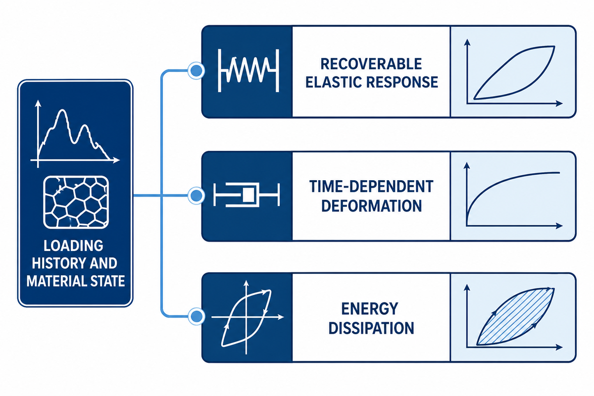
A viscoelastic material stores part of the work used to deform it and dissipates another part, rather than storing and returning all of it. Which characteristic is predominant depends upon the test window. Therefore, describing such a system as “solid-like” or “liquid-like” reflects the system at a particular instance, and doesn’t imply that the system is of that type. For Tengyang, this vocabulary frames evidence, consistent with the Lakes Lab notes; it is not a grade claim.
An ideal solid, treated as a purely elastic material, responds immediately when a load is applied, returns the stored energy, and reaches its original state when the load is removed. Under applied stress, a viscous fluid keeps deforming and doesn’t allow any flow to be recovered. Polymer behavior between the above-mentioned ideals is attributable to the presence of molecular segments. Molecular segments take some time to rearrange.
Viscoelastic properties become more intelligible when elastic properties and viscous properties are interpreted as response ideals for elasticity and viscosity rather than as limiting constituents of a mixture, which improves an understanding of viscoelasticity. Elasticity and other elastic characteristics describe the recoverable part of the response; the viscous component and other viscous and elastic properties account for time-dependent dissipation, storage, or flow. As such, the statement “polymer is viscous and elastic” is obviously oversimplified. In search language, “viscoelasticity materials” usually refers to viscoelastic materials, while “viscoelasticity properties” refers to material properties that vary with time, temperature, and rate. For a more realistic analysis, consider the limiting conditions defined independently by strain rate, temperature, and the duration of the response observation window.
| Response | During load | After unloading | What must be stated |
|---|---|---|---|
| Ideal elastic | Immediate deformation | Immediate recovery | Load and modulus definition |
| Ideal viscous | Continuous flow | No recovery of accumulated flow | Stress, time, temperature, and viscosity |
| Viscoelastic | Immediate plus delayed response | Immediate, delayed, and possibly incomplete recovery | Full loading history and material state |
Universities characterize viscoelastic behavior, meaning the behavior of viscoelastic materials, through time-dependent stress and strain functions rather than by a “percentage solid” classification [1]. The same polymer may therefore look nearly elastic in a short, cool observation and much more dissipative during a longer or warmer one. With a slower or longer observation, or at high temperature, that polymer could appear very dissipative. It should be clarified that the type of the material hasn’t changed. Here, the observation has become longer; more generally, its clock has changed.
Biomaterial and biomechanics research also uses viscoelasticity measurement methods, but human tissue is outside this guide’s industrial polymer and adhesive scope. Terms common to both systems don’t allow biological acceptance criteria to be adopted for a synthetic polymer or an adhesive. Nor do the shared terms make biological acceptance criteria transferable to a synthetic polymer, an adhesive layer, or a bonded assembly. When studying viscoelasticity, a viscoelastic liquid cannot be reduced to the viscosity of the material because that value describes only its flow component.
Time, Temperature and Rate Change the Observed Response in Viscoelasticity
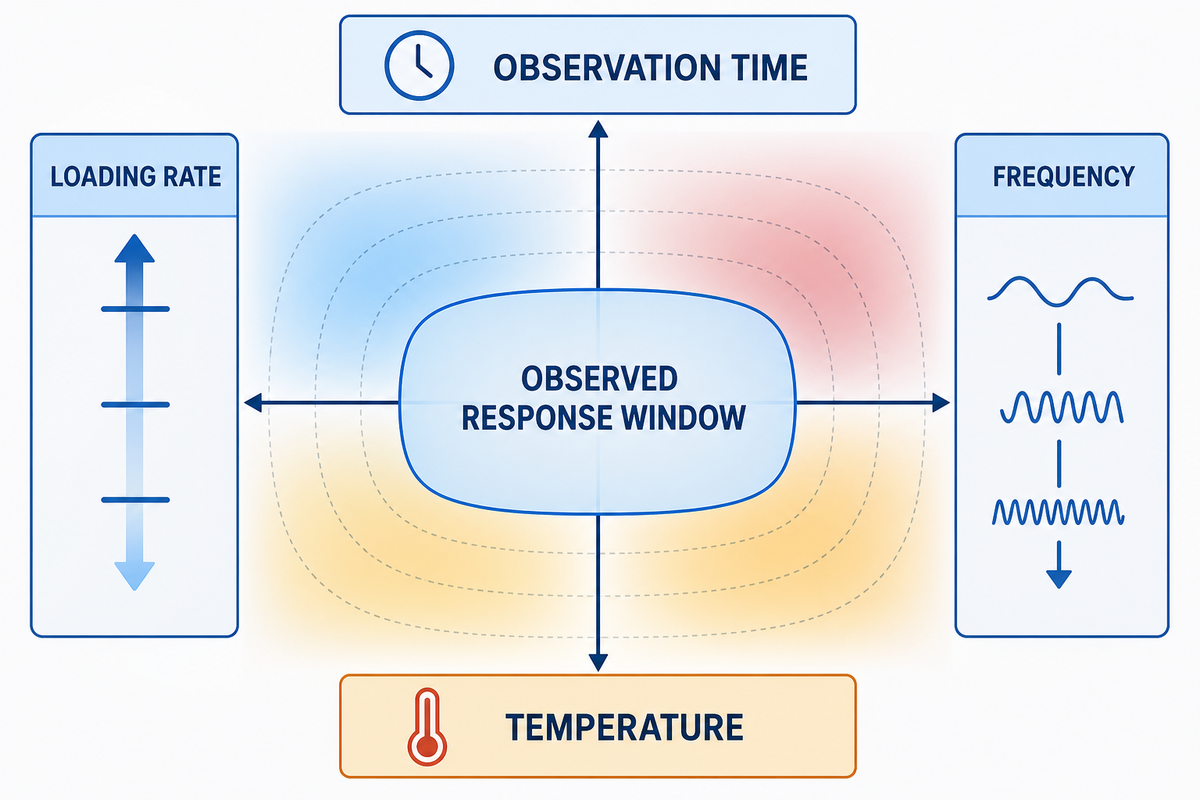
Here, the Observed Response Window in Viscoelasticity is the time scale on which loading, molecular rearrangement, and observation compete, as illustrated by the NIST viscoelastic-property reference. In a fast test, molecular segments may not have time to move to more favorable positions, resulting in an appearance of molecular stiffness. Under a more relaxed observation or an elevated temperature, further rearrangement of molecular segments results in a more compliant (less stiff) and dissipative response. Such rearrangement of the segments would also result in energy dissipation.
One of the other methods for setting that clock is using frequency. At 10 Hz, an oscillation completes ten cycles each second, while at 0.5 Hz an oscillation gives the specimen far more time per cycle. On the other hand, 0.5 Hz oscillations happen only once every 2 seconds. Which one is “more right”? Neither. It all depends on what measurement window we want to work with, so long as the deformation remains in the linear region.
Key takeaway
Viscoelastic values are portable only when the material state, deformation mode, loading clock, temperature, and interpretation criterion travel with them.
While the relationship between temperature and time is discernible in some cases, other variables can affect how a polymer material functions, so temperature isn’t a universal conversion key. These variables include transitions, crystallization, moisture, physical aging, formulation changes, and other changes in a substance’s composition; they alter which molecular mechanisms are active. The best comparison is not simply “value A” versus “value B.” The term should be used only when assessing the same response metric under demonstrably comparable conditions, clocks, and material states.
A curve without its clock is not a material ranking. It is an observation with its context removed.
This principle explains why short-term stiffness shouldn’t be carried directly into a long hold and why a warm process result shouldn’t be treated as a cool service result without further evidence. Time, frequency and rate are all related to one another and so are temperatures; however, evidence needs to be provided to support the connection for the specific example and the extent of the relationship.
Creep and Stress Relaxation in a Viscoelastic Solid
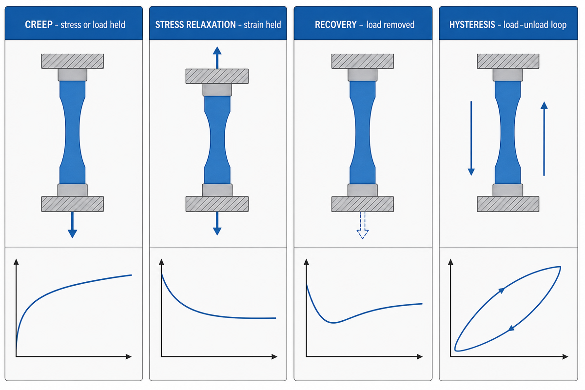
Creep and stress relaxation are different kinds of experiments, but they use similar principles. Creep is used to evaluate time-dependent strain under sustained stress, and stress relaxation is used to evaluate how stress decreases under constant strain. Calling stress relaxation the opposite or inverse of creep is misleading because it focuses on the changing output and hides the controlled experimental input.
| Experiment | Controlled input | Measured output | Question answered | Common limit |
|---|---|---|---|---|
| Creep | Stress or load | Strain or displacement over time | How deformation accumulates during a hold | Fixture and geometry may prevent constant specimen stress |
| Stress relaxation | Strain or displacement | Stress or force over time | How holding force decays at fixed deformation | Machine compliance may change actual strain |
| Recovery | Load removed after a defined history | Recovered and residual strain | What portion returns, and how fast | Too short a recovery window hides delayed recovery |
| Hysteresis | Load-unload cycle | Loop area and path | How much work is dissipated in that cycle | Rate, amplitude, and heating affect the loop |
Brown’s linear-viscoelasticity chapter defines creep compliance as strain response to a step of stress and relaxation modulus as stress response to a step of strain.[1] In the framework of good practice, rheology states that a measurement designed for linear interpretation should remain within the limits of the linear region of the viscoelastic material, and the temperature should be controlled.[2]
Under a constant hanging load, a bonded strip allows observation of creep effects. If a second strip is then clamped at a fixed displacement, the load at that second strip will be observed to decrease, which is the stress relaxation effect. Neither the creep nor stress relaxation effects prove service life or interface failure. Further data are required, including the environment, recovery, geometry, temperature, and how the material failed.
Reports should assess whether constant stress is appropriately demonstrated, indicate how applied stress or applied force is calculated, and determine the mode of deformation as tension, compression, bending, or shear. Reports of shear stress can’t be compared directly with tensile results unless a valid conversion and its assumptions are supplied. These aspects are pertinent to the analysis because compliance of fixtures and other features can result in the specimen being deformed in a manner different from the prescribed deformation.
What the Classic Viscoelastic Models Can and Cannot Explain
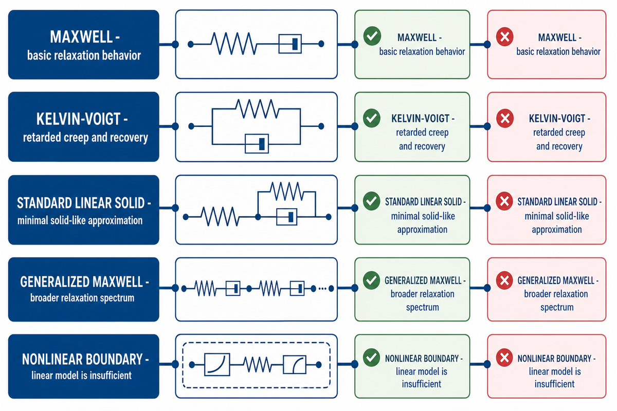
A spring in a spring-and-dashpot model embodies an ideal elastic contribution, as developed in the Brown University-hosted linear-viscoelasticity chapter. Element arrangement in the model determines which creep, relaxation, and recovery features the model reproduces within a fitted range. These elements are analogies, not literal microscopic structures or universal material laws.
| Model | Creep response | Stress relaxation | Useful for | What it misses |
|---|---|---|---|---|
| Maxwell | Immediate elastic strain plus continuing viscous strain | Exponential decay in the ideal step case | Basic relaxation behavior | Bounded long-time creep of a solid |
| Kelvin-Voigt | Delayed, bounded deformation | No instantaneous step-strain response in its simplest form | Retarded creep and recovery | Immediate elastic jump |
| Standard linear solid | Immediate plus delayed bounded response | Decay toward a nonzero equilibrium modulus | A minimal solid-like approximation | Broad or multiple relaxation spectra |
Brown’s chapter and the University of Wisconsin-Madison notes show why model choice must follow the response feature being represented.[1][3] A good fit doesn’t turn a dashpot viscosity into a unique molecular identity, nor does it prove that identical parameters apply outside the fitted temperature, time, frequency, or strain range.
It’s well known that real relaxation processes can’t be ideally represented by a few parameters. A good fit is useful only when the model’s representation of the measured mechanical behavior predicts a held-out response. Reporting should therefore cover the loading mode, strain range, fitting window, parameter units, optimization method, and residual pattern.
Maxwell model behavior includes a characteristic relaxation time. By contrast, the standard linear solid model, or Zener model, introduces a nonzero long-time elastic contribution. Compact models consider elastic moduli and viscosity parameters. However, they don’t eliminate dependence of the elasticity parameter on the boundaries of the modeled domain. Parameters with the same name may represent different physical quantities or fitting options in different cases.
| Response type or model class | Representation | Useful interpretation | Boundary to report |
|---|---|---|---|
| Ideal elastic limit | Immediate, fully recoverable response | A reference limit for stored energy | It does not represent delayed flow or dissipation |
| Ideal viscous limit | Continuing deformation under stress without elastic recovery | A reference limit for dissipative flow | Stress, time, temperature, and viscosity remain part of the result |
| Maxwell model | Spring and dashpot in series | Stress relaxation and a fluid-like long-time limit | It does not retain a nonzero equilibrium modulus |
| Kelvin-Voigt model | Spring and dashpot in parallel | Delayed creep toward a bounded strain | It does not reproduce an instantaneous strain jump |
| Standard linear solid or Zener model | Elastic and viscous elements with an equilibrium elastic contribution | Bounded creep and relaxation in one compact model | Parameters apply only inside the fitted material and condition range |
| Generalized Maxwell series | Multiple relaxation branches | A broader relaxation spectrum than a single branch | Report parameter count, fitting window, residuals, and held-out validation |
| Linear viscoelastic material | Response remains proportional inside a demonstrated linear region | Linear superposition and compact modelling may be useful | Amplitude sweep, mode, temperature, and loading clock must travel with the result |
| Nonlinear or viscoplastic boundary | Large-strain response, structural change, or permanent flow | Signals that a linear model alone is insufficient | Recovery, repeat cycles, self-heating, and thermal history require separate evidence |
Linear and Nonlinear Viscoelasticity
Linear behavior of viscoelasticity refers to the response of a material to a given load, where the response of the material is proportional to the load. Such behavior allows the usage of linear models. In case of nonlinear behavior, the shape or the response of the material may not be proportional to the load. This behavior depends on the material and the condition of the load, and isn’t limited to a given value.
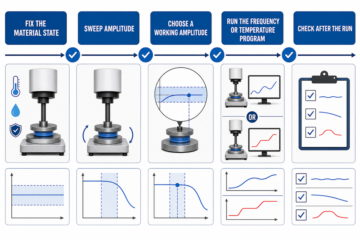
ISO 6721-1:2019 addresses dynamic mechanical properties of materials within linear viscoelastic behavior and qualifies when flexural and tensile measurements are comparable.[4] In oscillatory work, an amplitude sweep is commonly used to locate a region where storage and loss measures remain suitably stable before a frequency sweep is interpreted.
- Fix the material state: record formulation, conditioning, age, geometry, and temperature before changing amplitude.
- Sweep amplitude: identify the window in which the selected response measures remain acceptably independent of amplitude.
- Choose a working amplitude: stay inside that window with margin for repeatability and instrument limits.
- Run the frequency or temperature program: keep deformation mode and material state consistent.
- Check after the run: look for drift, self-heating, damage, crystallization, or other evidence that the specimen changed.
Viscoelastic response can include delayed recovery, while viscoplastic response includes permanent deformation or flow after the relevant loading condition is reached. Viscoplasticity is a separate boundary question, and the reverse relationship may not hold. Materials may exhibit both types of behavior, and a loading/unloading curve may not differentiate between them.
How DMA and Rheology Characterize Viscoelastic Behavior
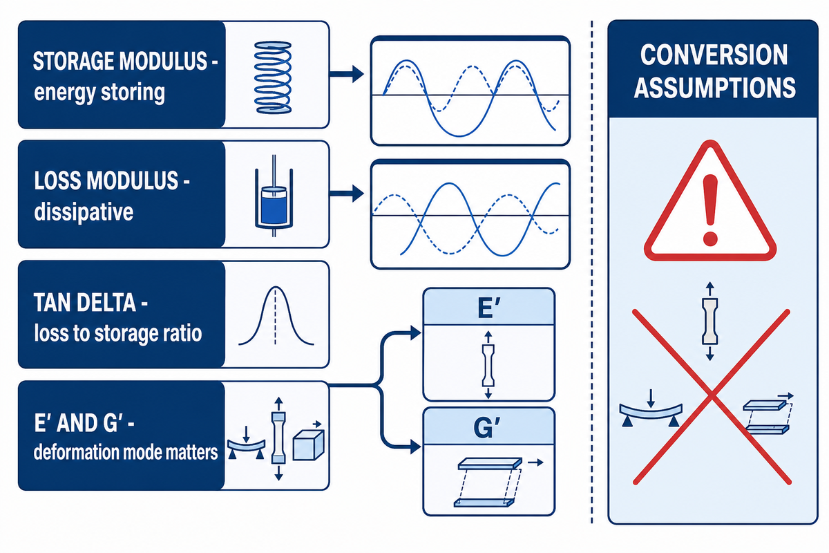
Dynamic mechanical analysis and oscillatory rheology techniques involve applying stress or strain periodically, measuring the input and output, and analyzing storage and loss. Storage modulus represents the in-phase, energy storing part, while loss modulus is out-of-phase and dissipative. For the given deformation case, the ratio of loss modulus to storage modulus yields the value of tan delta.
For a tensile or bending dynamic mechanical test, reports commonly use E′ and E″. In oscillatory shear, they commonly use G′ and G″. These aren’t automatically interchangeable. A Caltech-hosted critical review explains that viscoelastic Poisson’s ratio can vary with time or frequency and is difficult to measure accurately.[5] Any conversion must state assumptions such as homogeneity, isotropy, linearity, and the conversion data used.
A TA Instruments DMA training example lists an ABS specimen as 50.0000 mm × 12.9100 mm × 3.1700 mm. Its strain-sweep graphic uses storage-modulus scale marks at 0.1 MPa, 1 MPa, 10 MPa, 100 MPa, and 1,000 MPa. The same training deck shows a separate PC temperature-ramp example from -150 °C to 180 °C at 3 °C/min, 1 Hz, and 15 µm amplitude; these figures are study-specific settings, not material specifications or acceptance limits for Tengyang products.
| Reported item | Physical reading | Typical unit | Context required | Does not prove |
|---|---|---|---|---|
| Storage modulus, E′ or G′ | In-phase stored response | Pa and scaled units | Mode, geometry, amplitude, frequency, temperature | Universal stiffness rank |
| Loss modulus, E″ or G″ | Out-of-phase dissipative response | Pa and scaled units | Same conditions plus signal quality | Failure mechanism |
| tan δ | Loss modulus divided by storage modulus | Dimensionless | Mode, frequency, temperature, peak criterion | A unique glass-transition temperature |
| Phase angle, δ | Lag between periodic input and response | Degrees or radians | Waveform, convention, and linearity | Material identity |
Transition assignment adds another layer. ASTM E1640-23 states that glass transition occurs over a range and that an assigned value may vary with technique; in ideal cases, the onset of storage-modulus decrease marks the transition.[6] ISO 6721-11:2019 describes determination from dynamic properties during linear heating.[7] A report should therefore say whether it used storage-modulus onset, loss-modulus peak, tan-delta peak, or another stated criterion.
NIST’s contact-resonance work adds a scale and acquisition warning: agreement with time-temperature-superposed low-frequency dynamic data depended on acquisition mode and scanning velocity.[8] Instrument output is evidence only inside the method, sampling, and analysis chain that produced it.
Pay attention to a few things when examining dynamic reports. These include the deformation mode (tensile, flexural, or shear), the axis scale (linear or logarithmic), the scan variable (temperature, frequency, or both), and whether the test is static or dynamic. Generally, a repeatable measurement and a peak in the correct position do not justify converting E and G without recording the assumed Poisson’s ratio and its frequency or temperature dependence. Isolating a trace or obtaining replicate measurements can help determine whether a peak reflects material properties or a measurement artifact. When converting E and G, any assumed value, especially Poisson’s ratio and its frequency or temperature dependence, should be included in the calculation record.
Time-Temperature Superposition and Its Limits
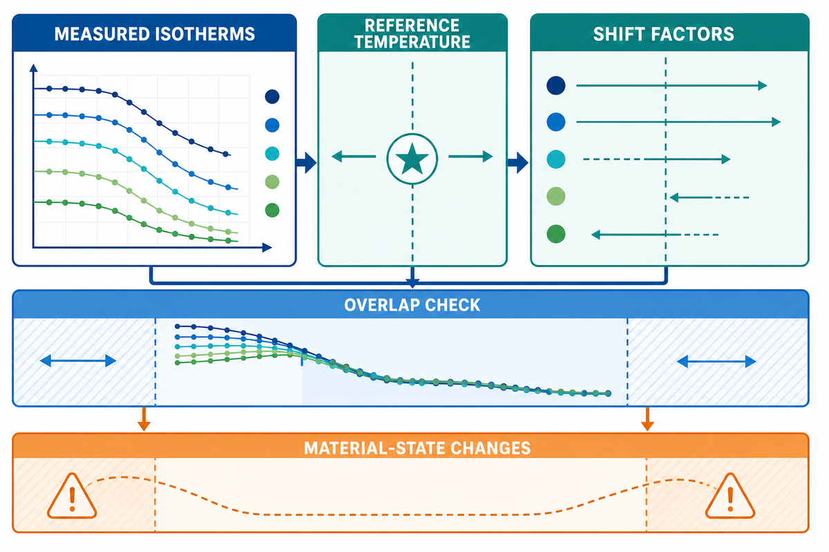
Time-Temperature Superposition (TTS) uses response data measured at several temperatures to generate a master curve at a single reference temperature. Data taken at different temperatures over overlapping time or frequency domains are shifted to a reference temperature to build a master curve for the material’s response window. This method can extend the represented time or frequency window, but only when the material is sufficiently thermorheologically simple across the selected range and the shifted regions overlap consistently.
Measured isotherms must be presented along with the measured window. Reference-temperature definition must be provided. Reports should state and apply the shift factors, and inspect overlap separately for each response metric. Possible material-state changes, including moisture loss, crystallization, physical aging, self-heating, degradation, or a second transition, must be discussed for the test period.
Do
- Keep raw isotherms and measured limits
- Report reference temperature and shift method
- Inspect storage and loss results separately
- Check aging, moisture, heating, and transitions
Don’t
- Treat smooth overlap as universal validity
- Hide the extrapolated region
- Transfer shift factors across formulations
- Call a master curve a service-life guarantee
A 2024 study of dry and 50% relative-humidity-conditioned PA6 and 50 wt% short-glass-fibre PA6 found that simple equivalence models didn’t capture thermal-history effects, and that self-heating produced deviations at large strain. DOMO Chemicals supplied the tested plates, and one of the company’s employees was a co-author.[9] This is a bounded counterexample, not proof that all PA6 systems or all master curves fail.
Another limit appears in a NIST-hosted PEN study. Longer physical aging exposed a second relaxation mechanism that invalidated time-aging superposition; increasing temperature also revealed two mechanisms and lack of thermorheological simplicity.[10] Material state can evolve, so “conditioned” should include time and history, not only a nominal temperature.
For one constructive example, a 2026 PC/ABS study measured 0.5 to 10 Hz, excluded its 0.5 Hz series from quantitative trend analysis because the transition region had insufficient sampling, and reported a storage-modulus master curve at a 115.8 °C reference temperature using the remaining frequencies. Minor scatter remained in the loss modulus.[11] That example shows why a master curve can be satisfactory for one metric without validating every response. For adjacent context, see glass-transition measurement conventions.
A bounded study-window example
Figures below represent a 2026 PC/ABS experiment and illustrate how measurement envelopes, exclusion rules, and metric-specific outcomes should be reported. Those figures shouldn’t be interpreted to set requirements for hot-melt adhesive films, other PC/ABS resins, or any products made by Tengyang.
| Reported element | Study value | Reading boundary |
|---|---|---|
| Measured frequency window | 0.5 Hz to 10 Hz | Five measured series, not an unlimited frequency range |
| Series retained for quantitative trends | 1 Hz, 2 Hz, 5 Hz, and 10 Hz | The 0.5 Hz series had only 94 points and insufficient transition-region sampling |
| Reference temperature | 115.8 °C | A study choice, not a universal reference temperature |
| Approximate glassy plateau | 1,800 MPa | Applies to the reported PC/ABS system and method |
| Approximate rubbery plateau | 5 MPa to 10 MPa | Not a specification or acceptance range |
| Storage-modulus result | Shifted over about five decades | Validity remains tied to the retained data and model assumptions |
| Loss-modulus result | Minor scatter remained | One satisfactory metric does not validate every metric |
| Model-development set | 3,751 samples | Sample count does not erase chemistry and domain limits |
Measurement examples are classified as information that’s measured, retained, shifted, and/or predicted. Distinguishing this information is important, because a curve that fits the data perfectly may conceal a series that has been excluded from the analysis, or a transition region that’s data poor. A report should provide raw measurement data, mark exclusions, distinguish interpolation from extrapolation, and state which response metric has met the chosen acceptance criterion.
From Curve Context Evidence to Allowed Inference: Sample State and Measurement Context
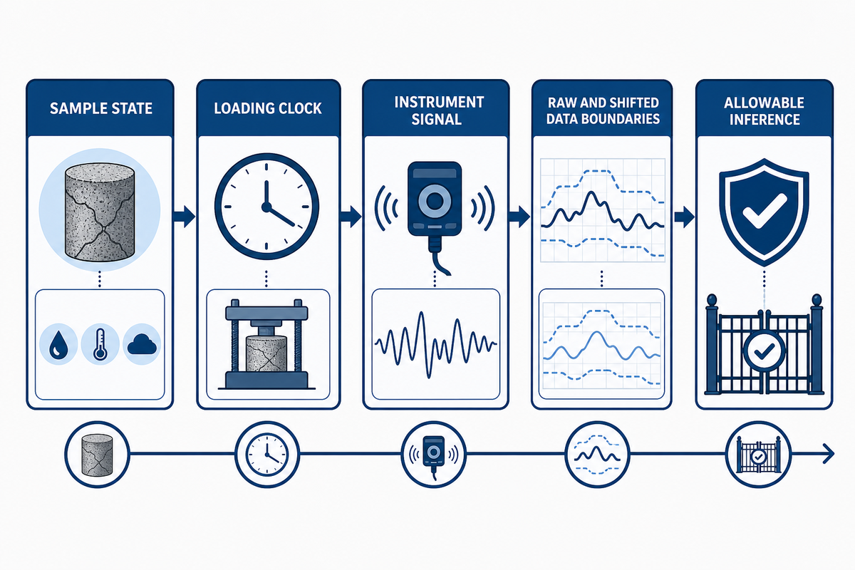
Read the evidence ladder from left to right: establish the material and specimen history, define the deformation mode, geometry, amplitude, time or frequency, temperature, and conditioning, then inspect the instrument context, data treatment, and uncertainty before interpreting any curve or modulus value. Each measurement should also state the analysis criterion and a basis for uncertainty. This evidence ladder groups raw measurements, transformed views, and allowed inferences rather than treating them as interchangeable checklist items; it is an interpretation aid, not a standard.
| Stage (chain stage and evidence category) | Evidence category (why it matters in the dependency) | Why it matters / what its absence prevents | Evidence to retain or request |
|---|---|---|---|
| Sample state | Material identity and lot | Without the material boundary, differences cannot be assigned confidently to formulation or lot | Grade, lot, and composition boundary |
| Sample state | Specimen history and conditioning | Preparation, processing, moisture, storage, and aging can change the state being measured | Dimensions, preparation notes, processing history, and conditioning log |
| Loading clock | Deformation mode, geometry, and modulus type | Tension, bending, and shear are not automatic equivalents | Fixture, specimen dimensions, and E or G designation |
| Loading clock | Amplitude and linear-region proof | Excess amplitude can change the response and invalidate a linear-model interpretation | Amplitude sweep and selected working point |
| Loading clock | Frequency, time, rate, and temperature | These conditions define the observation window and limit window-to-window comparison | Full loading program and measured range |
| Instrument signal | Instrument and calibration context | Compliance, force range, and calibration affect the recorded signal | Instrument identity, calibration record, and compliance correction |
| Instrument signal | Raw and shifted data boundaries | Measured, shifted, interpolated, and extrapolated regions do not carry the same support | Raw isotherms, shift factors, and overlap |
| Instrument signal | Repeatability, exclusions, and processing choices | A clean curve can hide scatter, excluded runs, smoothing, or transformations | Replicates, raw data, excluded runs, and processing record |
| Allowable inference | Transition criterion and model boundary | Onsets, peaks, and fitted models answer different operational questions | Criterion, baseline method, model range, and residual pattern |
| Allowable inference | Uncertainty, acceptance rule, and decision | This boundary separates an observed result from a permitted comparison, ranking, or pass-fail decision | Uncertainty estimate, range limits, and decision rule |
To see why the fields travel together, consider two purely illustrative report labels, not recommended settings. Report A might state a 2 mm specimen, 0.1% strain at 1 Hz and 23 °C after 24 hours at 50% relative humidity. Report B might state a 3 mm specimen, 1% strain at 10 Hz and 60 °C after 7 days of conditioning. A numerical difference between those reports can’t be assigned to formulation alone because geometry, amplitude, clock, temperature, and conditioning all changed. The correct next action is to align the test contexts or limit the conclusion.
Use the chain before ranking formulations, suppliers, or test runs. If two reports use different modes or transition criteria, the next action isn’t to declare a winner. It’s to align the methods or state the limits of comparison. This same discipline applies when you compare bonding test reports.
This approach is different from a process-input checklist. Here, the focus is on the evidence rather than the decision. It doesn’t guide material selection or decision making regarding the format (film or powder) of the adhesive. It’s expected that these considerations would occur only after the evidence has been defined.
From Test Data to Adhesive Decisions
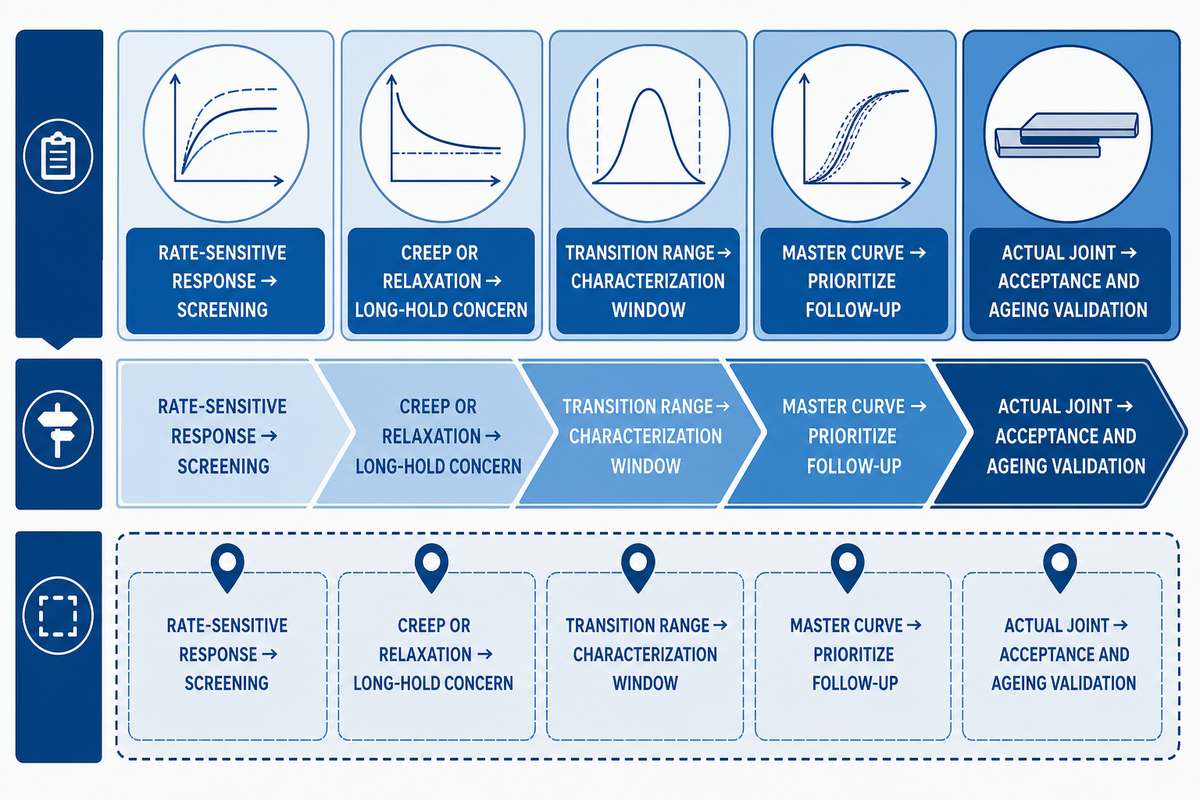
Viscoelastic measurements provide data on the response of a bulk material over defined periods of time and at various temperatures and rates. These measurements define response windows; the Curve Context Chain shows how sample state, loading clock, and signal handling constrain interpretation, but it does not itself select adhesives. Viscoelastic measurements, alone, don’t define the durability of a joint or the service life of a product. These attributes require data from the actual substrate, joint, and product system rather than from a surrogate system.
| Signal | Decision it can support | Evidence still required |
|---|---|---|
| Rate-sensitive storage and loss response | Choose conditions for further screening | Process-window and joint tests on actual substrates |
| Creep or relaxation under a stated hold | Identify a potential long-hold concern | Joint geometry, interface, environment, and failure-mode data |
| Transition range or damping peak | Define a characterization window | Application acceptance limits and ageing validation |
| Master curve inside a validated range | Prioritize additional test times or frequencies | Held-out validation and service correlation |
In a Sandia-led study, humid epoxy napkin-ring joints illustrate the boundary. Surface preparation, abrasion, and corrosion affected moisture-related strength loss; when surface-specific mechanisms were active, strength fell below the loss associated with bulk adhesive glass-transition depression and didn’t recover on drying.[12] That result belongs to the tested epoxy joint system, but the inference lesson is broader: bulk response can’t stand in for interface evidence.
For an adhesive project, carry the substrate pair, surface state, bond-line geometry, process history, service load and duration, environment, and acceptance method into the test plan. Use peel-test geometry and reporting when peel is relevant, and keep surface energy and wetting separate from bulk modulus.
After those boundaries are clear, the existing Tengyang solution page can help connect viscoelastic polymer response for adhesive selection with material format and application inputs. This guide does not replace family-based screening, trial planning, or qualification.
What Is Changing in Viscoelastic Characterization
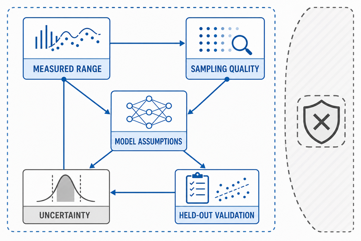
Verification depth and breadth are important for future prediction, which remains bounded by chemistry, measured range, sampling quality, model assumptions, and uncertainty. Artificial Intelligence won’t necessarily replace testing. Rather, its predictions will be constrained to the chemistry, measured range, sampling quality, model assumptions, and uncertainty under which tests are done. Evidence and rigor will be required to ensure the models are built for relevant temperature and frequency range.
The 2026 PC/ABS study used four frequency series to create 3,751 samples for model development, evaluated temperature-blocked cross-validation, and tested held-out-frequency behavior.[11] It also excluded an inadequately sampled 0.5 Hz series from quantitative trend analysis. That exclusion is as important as the model: more measured points don’t automatically become better evidence.
Model-assisted curves for engineering reports should identify training and validation ranges, held-out conditions, exclusions, uncertainty, and failure cases. They may be useful for planning tests. They don’t warrant a materials grade, expand the scope of a standard, or replace the need to evaluate joints and services directly.
Frequently Asked Questions
What do you mean by viscoelasticity?
Answer
Viscoelasticity describes behavior that combines recoverable elastic response with time-dependent viscous response and energy dissipation. The balance is not a fixed percentage printed on a material label. It changes with loading rate, observation time, temperature, strain level, deformation mode, and material state, so every result needs its complete test context.
What is elastic vs viscoelastic?
Answer
An ideal elastic material deforms immediately under load and returns stored energy when the load is removed. A viscoelastic material can also recover, but part of its response is delayed and part of the input energy is dissipated. The specific practical distinction depends on the tested time and temperature window.
What is an example of a viscoelastic fluid?
Answer
Polymer melts and some polymer solutions can behave as viscoelastic fluids because they flow while retaining a measurable elastic response over an appropriate time scale. The label is not a universal performance description. Molecular architecture, concentration, temperature, deformation rate, and measurement method determine which effects appear in the observed window.
What is the difference between viscoplasticity and viscoelasticity?
Answer
Viscoelasticity describes time-dependent response that can include delayed recovery. Viscoplasticity includes permanent deformation or flow after the relevant loading condition is reached. Real materials can show both, so unloading, recovery time, and repeat-cycle data are needed before assigning either behavior from a single loading curve.
What are some real-life examples of viscoelastic materials?
Answer
Common viscoelasticity examples include polymers, rubber-like solids, polymer melts, pressure-sensitive adhesive systems, biological tissues, and familiar foods, all of which show viscoelastic behavior. They’re examples, not equivalents. Different structures, loads, environments, and time scales govern a tendon, a polymer melt, and an adhesive layer. The useful comparison identifies the relevant response, such as creep, relaxation, damping, recovery, or flow, and then defines the measurement window. A shoe cushioning material may be judged by cyclic damping and recovery, while a sealed joint may be more sensitive to long-hold relaxation. A melt-processing question may instead focus on shear rate and flow. A material name alone can’t supply that context, and familiar behavior should never replace a stated test method.
Can viscoelasticity predict how long an adhesive bond will last?
Answer
No. Viscoelastic data can reveal time-, rate-, and temperature-sensitive bulk response, but bond life also depends on the interface, substrate preparation, joint geometry, load history, moisture, chemicals, ageing, and failure mode. Service-life statements need a validated relationship between the laboratory method and the actual bonded assembly. Useful evidence normally combines bulk characterization with joint-level testing under relevant environmental and loading histories, records where failure occurs, and checks whether accelerated conditions preserve the same mechanism. A master curve can help choose follow-up test windows; it isn’t, by itself, a lifetime warranty.
References & Sources: Evidence Boundaries
The attached documents correlate to the methods described, and provide third party definitions and examples. They are not certifications, patents, accredited laboratory results, or grade-performance data of Shanghai Tengyang New Materials Technology Co., Ltd. The examples provided show specific numbers. Study-specific numbers remain attached to the material, specimen, and test conditions reported by each source.
- Essentials of Linear Viscoelasticity, Brown University-hosted chapter.
- Good practice in rheological characterization.
- Viscoelasticity notes from the University of Wisconsin-Madison Lakes Lab.
- ISO 6721-1:2019 official catalogue record.
- Poisson’s Ratio in Linear Viscoelasticity: A Critical Review.
- ASTM E1640-23 official active standard page.
- ISO 6721-11:2019 official catalogue record.
- NIST viscoelastic property mapping publication record.
- 2024 PA6/GPA6 study on hygro-thermal history and viscoelastic modelling.
- NIST physical-aging study of amorphous PEN film.
- 2026 multi-frequency PC/ABS characterization study.
- OSTI record for the Sandia-led adhesive-joint degradation study.
Discuss the Evidence Needed for Your Bonding Trial
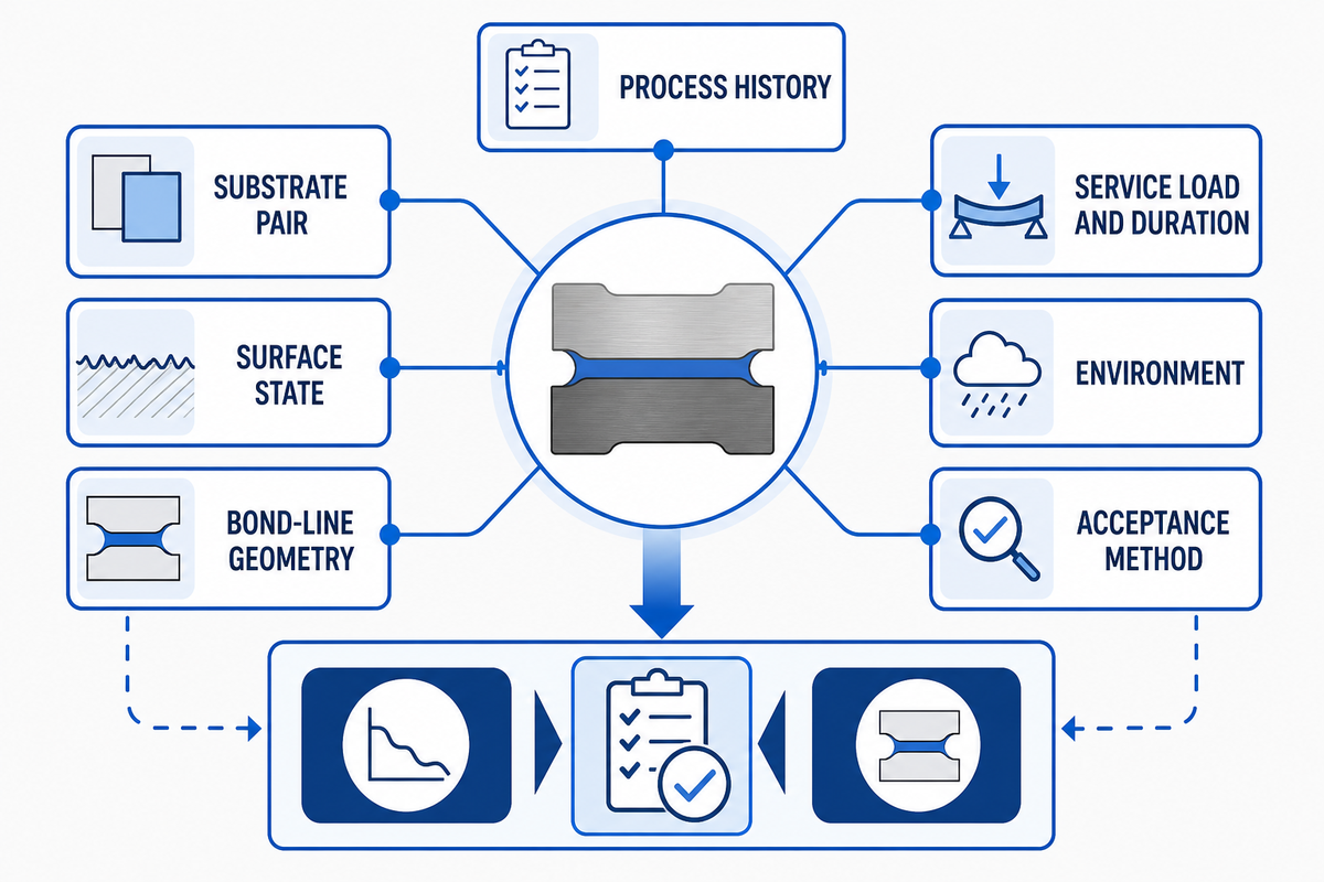
Discuss with Shanghai Tengyang the conditions under which the bond will be evaluated (i.e. temperature, humidity, load, and time, among others), using the NIST measurement reference as one public evidence point, and how the bond will be evaluated (i.e. direct observation, a defined test method, and a stated acceptance criterion). The evaluation of a joint may be informed by viscoelastic curves, but it still requires testing of the actual substrate and joint system. Hot-melt adhesive film, web, powder, or granule options may be discussed for the planned evaluation.
ABOUT TENGYANG
Industrial hot melt adhesive materials for bonding routes
Shanghai Tengyang New Materials Technology Co., Ltd. supports material discussions for production teams working with bonded products.
Available forms: hot melt adhesive film, web, powder and granules. Material families: TPU, EVA, PA, PES and PO.
CONTACT PROFILE
Betty Fang
Contact for material inquiries.